Documentation / Tutorial
1. Definition of waveguide geometry
Use a text editor to create a file called fiber.mgp:
# 'Background index' = refractive index at z -> +infinity
n 1.5
# Circular interface:
# outside index = 1.5, inside index = 3.5,
# center ρ = 0, center z = 0, radius = .16 microns
c 1.5 3.5 0 0 .16
# Define 'core area', explained below
C -.2 -.2 .2 .2
x
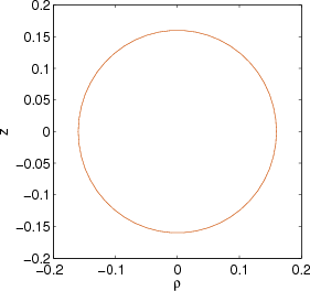
This is a simple waveguide-geometry file for wgms3d representing a fiber of .16 microns radius and a refractive
index of 3.5 embedded in a surrounding medium of refractive index 1.5. The lines starting with '#' are
simply comments, you may leave them out. The 'x' marks the end of the input file.
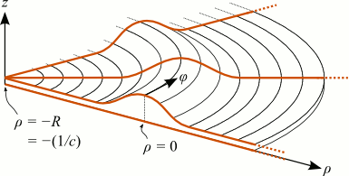
The two-dimensional waveguide cross section is spanned by the lateral ("horizontal") ρ axis and by the
vertical z axis (figure).
The line beginning with 'C' defines an area and is optional for our first calculations. It is only
required later for leakage / curvature calculations where the mode fields may have both real and imaginary
parts. In those cases wgms3d multiplies the whole mode field with a constant phase factor such that the mode
field in the area defined by 'C' is approximately real (this has no physical significance, but is
useful vor visualization purposes). The syntax is 'C ρ1 z1 ρ2 z2', meaning an area spanned by
the lower left point (ρ,z)=(ρ1,z1) and the upper right point (ρ2,z2).
2. Plot the waveguide geometry in Matlab
For a first check whether you've entered the geometry correctly, start up Matlab, change the current directory
to that where fiber.mgp resides, and make sure the matlab subdirectory from the wgms3d
distribution is in Matlab's search path (e.g., using the menu "File" - "Set Path..." or the addpath
command). Then type
>> wgms3d_plot_mgp('fiber.mgp')
at the Matlab prompt. This should open a figure and show the boundaries of the dielectric interfaces you have
defined.
3. Run wgms3d to calculate the modes
Open a terminal, change the current directory to that where fiber.mgp resides, make sure wgms3d is in
your search path, and run
$ wgms3d -g fiber.mgp -l 1.55 -U -0.8:120:+0.8 -V -0.8:120:+0.8 -n 4
These command-line arguments have the following meaning:
- -g fiber.mgp specifies the waveguide-geometry file
- -l 1.55 specifies the wavelength (1.55 microns)
- -U -0.8:120:+0.8 specifies the horizontal (ρ-axis) discretization grid, here: 120 uniformly
spaced points between -0.8 and +0.8 microns. (you can specify arbitrary non-uniform grids, too, see the
example in the tests/silicon_strip_waveguide/ subdirectory in the wgms3d distribution)
- -V -0.8:120:+0.8: same for the vertical (z-axis) grid.
- -n 4 tells wgms3d to calculate the 4 modes of the structure with the largest effective index (or
propagation constant).
After a few seconds you should get an output like this:
* wgms3d version 0.8.8 *
Curvature = 0.000000e+00/UOL (Radius of curvature = infUOL)
Wavelength = 1.550000e+00UOL; real calculation.
Setting up FD system matrix (initial dimension = 28800)...
Storing 192/14400 non-standard diffops (~0MB).
Eliminated 480 unknowns with Dirichlet BCs.
Final matrix dimension is 28320; 255488 non-zero entries.
Searching for modes near n_eff = 3.500
Factorizing system matrix using SuperLU... (~41MB)
Eigensolving using ARPACK (nev=4, ncv=20)...
Eigencalculation finished successfully (niter=8,nconv=4).
EV   0: n_eff = 1.9829687310274806 + i 0.0000000000000000e+00
        alpha = 0.00e+00dB/UOL [0.00e+00dB/90deg], pol = '?'
EV   1: n_eff = 1.9829687310274784 + i 0.0000000000000000e+00
        alpha = 0.00e+00dB/UOL [0.00e+00dB/90deg], pol = 'H'
EV   2: n_eff = 1.4516481956262905 + i 0.0000000000000000e+00
        alpha = 0.00e+00dB/UOL [0.00e+00dB/90deg], pol = '?'
EV   3: n_eff = 1.3396497677681698 + i 0.0000000000000000e+00
        alpha = 0.00e+00dB/UOL [0.00e+00dB/90deg], pol = '?'
Total walltime (min:sec) = 0:04.
You can see the four modes listed with their effective indices. The first two modes (0 and 1) have
approximately the same index of 1.98 -- those modes correspond to the two polarizations of the fundamental mode
of the circular fiber (which, in theory, should have identical effective indices; but remember this is
an approximate numerical solution)
Furthermore, wgms3d has generated several output files, namely x.txt, y.txt, and (most
importantly) hr-XX.bin and hz-XX.bin which contain the ρ and z components of the magnetic
field of the waveguides modes (XX = 00, 01, 02, 03).
4. Visualize the result
To have a look at the modes, go back to your Matlab session and type
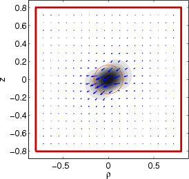
>> wgms3d_plot_ht(0, 'Geometry', 'fiber.mgp')
This should open a figure window and plot contours representing the magnitude of the transverse magnetic mode
field (in a linear scale), as well as arrows representing its vector direction; also the waveguide geometry is
included for clarity, and the boundaries of the computational domain are indicated by thick red lines.
The 'ht' in the last command stands for 'transverse magnetic field'; there are similar commands for
the transverse electric field (et), and for the longitudinal fields (hl and el),
however for these to work you have to instruct wgms3d to calculate and export those fields, too (command-line
options -E, -F, -G, and -H, respectively - just have a look at the help
output: wgms3d -h).
The wgms3d_plot_XX commands have a lot more options, which you can find by looking inside those
scripts. For example,
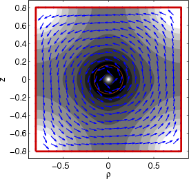
>> wgms3d_plot_ht(2, 'Geometry', 'fiber.mgp', 'LogContours', 1, 'QuiverGrid', 20, 'QuiverNormed', 'QuiverScale', 0.7)
gives you logarithmically spaced contours (here, in steps of 1 dB), makes the script re-interpolate the field
data such that you get 20 x 20 arrows (give an argument of 0 to QuiverGrid to disable
re-interpolation), and finally makes the arrows all have the same length instead of being proportional to the
magnitude of the local field.
This example shows mode #2: since its effective index of 1.451 is lower than the cladding index of 1.5, it
shouldn't be interpreted as a mode guided by the fiber. In fact, it is a mode guided by a metallic waveguide
with perfectly conducting walls (located at the borders of the computational domain) with a non-homogeneous
dielectric filling.
5. Calculating leaky modes with Perfectly
Matched Layers (PMLs)
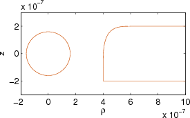
Let's create a waveguide structure fiberleak.mgp that supports leaky modes (even when the waveguide
itself is straight and not curved). To this end we take the fiber from above and add a little slab-like
structure with a large refractive index at the right-hand side - admittedly it's a bit absurd, but it shows you
how to create Bézier-type as well as straight dielectric interfaces:
n 1.5
c 1.5 3.5 0e-6 0e-6 .160e-6
b 1.5 3.5 .4e-6 -.1e-6 .4e-6 .2e-6 .6e-6 .2e-6
l 3.5 1.5 .4e-6 -.1e-6 .4e-6 -.2e-6
l 3.5 1.5 .4e-6 -.2e-6 100e-6 -.2e-6
l 1.5 3.5 .6e-6 .2e-6 100e-6 .2e-6
C -.2e-6 -.2e-6 .2e-6 .2e-6
x
The 'l' lines specify a linear (straight) dielectric interface. The syntax is 'l nleft nright
ρ1 z1 ρ2 z2', meaning a straight line from (ρ,z)=(ρ1,z1) to (ρ2,z2)
with refractive indices nleft and nright on the left-hand and right-hand sides of this line,
respectively (as seen when walking from point 1 to point 2).
The 'b' lines specify a three-point Bézier curve. The syntax is 'b nleft nright ρ1 z1
ρ2 z2 ρ3 z3'. (Internally, two more nodes are interpolated between points 1+2 and 2+3 to make sure
the local curvature is zero at the ends of the curve).
Now let's run wgms3d:
$ wgms3d -g fiberleak.mgp -l 1.55e-6 -U -0.8e-6:500:+2.3e-6 -V -1.0e-6:181:+1.01e-6 -n 4 -s 1.98 -P e:30:0.5
The new command-line arguments have the following meaning:
- -s 1.98 tells wgms3d to search for modes with an effective index in the neighbourhood of 1.98. This
argument is important, since otherwise wgms3d doesn't know which mode you're interested in; it would rather
output some 'spurious' modes whose fields are concentrated inside the PML region, which have no physical
significance but whose effective index is larger than 1.98 and thus would be preferably returned by the
eigenvalue solver.
- -P e:30:0.5 enables a PML absorbing layer at the 'e'ast side of the computational domain,
with a thickness of 30 discretization points, and whose strength is scaled by a factor of 0.5 relative to the
default 'optimum' PML strength given in the paper. Appropriate settings for this option depend on the
waveguide geometry and on the considered mode and must be found by trial-and-error, using the plot commands to
inspect the calculated modes and check them for obvious errors due to undesired reflections at the PML.
The computation now takes a bit longer and consumes more memory due to the larger number of discretization
points. The shell output looks something like this:
* wgms3d version 0.8.8 *
Curvature = 0.000000e+00/UOL (Radius of curvature = infUOL)
Wavelength = 1.550000e-06UOL; complex calculation.
Setting up FD system matrix (initial dimension = 181000)...
Storing 6745/90500 non-standard diffops (~18MB).
Eliminated 1362 unknowns with Dirichlet BCs.
Final matrix dimension is 179638; 1637546 non-zero entries.
Searching for modes near n_eff = 1.980
Factorizing system matrix using SuperLU... (~703MB)
Eigensolving using ARPACK (nev=4, ncv=20)...
Eigencalculation finished successfully (niter=7,nconv=4).
EV   0: n_eff = 1.9764099990630652 + i 1.0503532193893206e-02
        alpha = 3.70e+05dB/UOL [0.00e+00dB/90deg], pol = 'V'
EV   1: n_eff = 1.9917951427543028 + i 6.9603012322827194e-03
        alpha = 2.45e+05dB/UOL [0.00e+00dB/90deg], pol = 'H'
EV   2: n_eff = 1.8451030106630903 + i 1.4143695929151687e-01
        alpha = 4.98e+06dB/UOL [0.00e+00dB/90deg], pol = 'V'
EV   3: n_eff = 1.9190805395610866 + i 1.7529396517506088e-01
        alpha = 6.17e+06dB/UOL [0.00e+00dB/90deg], pol = 'V'
Total walltime (min:sec) = 1:23.
The output now also gives you the leakage losses in dB per unit of length (here, since the waveguide geometry
as well as the wavelength was specified in meters, the leakage losses are in dB/m). Furthermore, the two
previously degenerate fundamental modes of the fiber here split up into clearly distinguishable (predominantly)
horizontally and vertically polarized modes, with effective indices of 1.992 and 1.976, respectively.
To visualize the modes, go back to Matlab and enter:
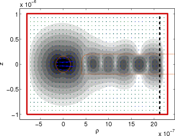
>> wgms3d_plot_ht(0, 'Geometry', 'fiberleak.mgp', 'LogContours', 3, 'RealContours')
Here, the RealContours option results in the contour plot to be based on the real part of the mode
field only, so that you can directly see the radiated field in the slab in the form of a spatial
oscillation. The radiated field is slightly non-uniform since several modes are excited in the slab due to the
asymmetry in its upper left corner. The beginning of the PML region on the right-hand (east) side of the
computational domain is marked with the thick black dashed line.
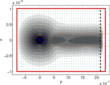
If you omit the RealContours option, the contours will display the absolute value of the
field:
>> wgms3d_plot_ht(0, 'Geometry', 'fiberleak.mgp', 'LogContours', 3)
The absolute value of the field corresponds to the radiation amplitude and does not significantly
oscillate. In this display mode you can clearly see how the PML damps the field without introducing a standing
wave in the slab due to parasitic reflections. This indicates that our PML settings are probably okay (neither
too weak nor too strong). (Try out what happens when you change the PML scaling from 0.5 towards much lower or
much higher values.)
6. Calculating curvature / bending loss
Curvature losses of waveguides are also easily calculated using wgms3d. We now go back to the original fiber
without the adjacent slab (fiber.mgp).
Use the '-R' option to specify a radius of curvature of the entire waveguides (and don't forget to
enable the PML):
$ wgms3d -g fiber.mgp -l 1.55 -U -0.8:200:+2.3 -V -1.5:201:+1.5 -n 4 -s 2.0
-P e:30:0.5 -P n:30:0.5 -P s:30:0.5 -R 1.7
Here's the shell output:
* wgms3d version 0.8.8 *
Curvature = 5.882353e-01/UOL (Radius of curvature = 1.700000e+00UOL)
Wavelength = 1.550000e+00UOL; complex calculation.
Setting up FD system matrix (initial dimension = 80400)...
Storing 15911/40200 non-standard diffops (~43MB).
Eliminated 802 unknowns with Dirichlet BCs.
Final matrix dimension is 79598; 1063083 non-zero entries.
Searching for modes near n_eff = 2.000
Factorizing system matrix using SuperLU... (~431MB)
Eigensolving using ARPACK (nev=4, ncv=20)...
Eigencalculation finished successfully (niter=26,nconv=4).
EV   0: n_eff = 2.0095819097943122 + i 5.8014472821806742e-03
        alpha = 2.04e-01dB/UOL [5.45e-01dB/90deg], pol = 'H'
EV   1: n_eff = 2.0102046955531518 + i 5.4406798460499154e-03
        alpha = 1.92e-01dB/UOL [5.12e-01dB/90deg], pol = 'V'
EV   2: n_eff = 1.9308346699396537 + i 4.3596398496773914e-01
        alpha = 1.54e+01dB/UOL [4.10e+01dB/90deg], pol = 'V'
EV   3: n_eff = 1.9434002331683438 + i 4.4616185694016069e-01
        alpha = 1.57e+01dB/UOL [4.19e+01dB/90deg], pol = '?'
Total walltime (min:sec) = 1:33.
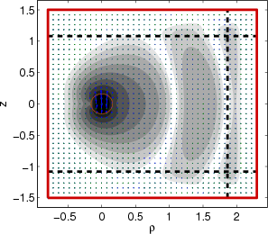
Plot the horizontally polarized mode in Matlab using
>> wgms3d_plot_ht(0, 'Geometry', 'fiber.mgp', 'LogContours', 3, 'QuiverGrid', 40, 'RealContours')
This time the losses are given, as above, in dB per unit of length (measured along the waveguide axis at
ρ=0), and additionally in dB per 90-degree bend (this is only the pure bending loss, not including any
effects due to transitions between straight and curved waveguide sections).
7. Calculating complex modes
It is well-known that some waveguide structures, even when they consist only of lossless dielectrics and
perfectly conducting metals, may have modes with a complex (i.e., neither purely real nor purely imaginary)
propagation constant. This can happen even if the waveguide is straight and does not have any obvious means for
energy to leak away from the waveguide core.
wgms3d can also be used to calculate these 'complex modes'. A PML is not necessary. Just run the mode solver
with the respective geometry; if complex modes are there, they will be returned just like any other mode.
Here, as an example, we consider the waveguide from Fig. 4b in J. Strube,
F. Arndt, "Rigorous Hybrid-Mode Analysis of the Transition from Rectangular Waveguide to Shielded Dielectric
Image Guide," IEEE Transactions on Microwave Theory and Techniques, vol. MTT-33, no. 5, May 1985:
n 1.0
l 1.0 2.449 -3.505e-3 -1      -3.505e-3 3.25e-3
l 1.0 2.449 -3.505e-3 3.25e-3 +3.505e-3 3.25e-3
l 1.0 2.449 +3.505e-3 3.25e-3 +3.505e-3 -1
C -3.0 0.0 +3.0 +3.0
x
and run wgms3d like this (the chosen wavelength corresponds to a frequency of 15 GHz):
$ wgms3d -g strube.mgp -l 19.986e-3 -U -7.899e-3:202:7.899e-3 -V 0:201:7.9e-3 -n 6
The resulting output (agrees well with the data of Fig. 4b in Strube's article):
* wgms3d version 0.8.8 *
Curvature = 0.000000e+00/UOL (Radius of curvature = infUOL)
Wavelength = 1.998600e-02UOL; real calculation.
Setting up FD system matrix (initial dimension = 81204)...
Storing 512/40602 non-standard diffops (~1MB).
Eliminated 806 unknowns with Dirichlet BCs.
Final matrix dimension is 80398; 727922 non-zero entries.
Searching for modes near n_eff = 2.449
Factorizing system matrix using SuperLU... (~142MB)
Eigensolving using ARPACK (nev=6, ncv=20)...
Eigencalculation finished successfully (niter=4,nconv=6).
EV   0: n_eff = 1.7301360663573013 + i 0.0000000000000000e+00
        alpha = 0.00e+00dB/UOL [0.00e+00dB/90deg], pol = 'V'
EV   1: n_eff = 1.0254521282951294 + i 0.0000000000000000e+00
        alpha = 0.00e+00dB/UOL [0.00e+00dB/90deg], pol = '?'
EV   2: n_eff = 0.6667567603225206 + i 0.0000000000000000e+00
        alpha = 0.00e+00dB/UOL [0.00e+00dB/90deg], pol = 'V'
EV   3: n_eff = 0.1577385548627442 + i-7.3456104855028093e-01
        alpha =-2.01e+03dB/UOL [0.00e+00dB/90deg], pol = '?'
EV   4: n_eff = 0.1577385548627442 + i 7.3456104855028093e-01
        alpha = 2.01e+03dB/UOL [0.00e+00dB/90deg], pol = '?'
EV   5: n_eff = 0.0000000000000000 + i 8.1605468406413462e-01
        alpha = 2.23e+03dB/UOL [0.00e+00dB/90deg], pol = 'H'
Total walltime (min:sec) = 0:12.
Modes #0, #1 and #2 are ordinary propagating modes of the waveguide, since their effective index is real. Modes
#3 and #4 are the complex modes whose computation we wanted to illustrate here. They always come in
complex-conjugate pairs. Mode #5 is an ordinary evanescent mode of the waveguide, since its effective index is
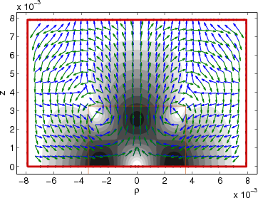
purely imaginary. Here we plot one of the complex modes:
>> wgms3d_plot_ht(3, 'Geometry', 'strube.mgp', 'QuiverGrid',
30, 'QuiverNormed', 'QuiverScale', 0.7)
In plots of complex-valued mode fields, the real and imaginary parts of the mode field are represented by blue
and green arrows, respectively.
8. Remarks
Some more things that deserve mention:
- The discretization grids in the examples above were not optimized in any way. In practice, you should
improve the discretization grid (as well as play with the PML settings) until the result you're interested in
(effective index, leakage losses, overlap integrals computed from the mode fields, etc.) does not change
significantly any more. It can happen that you need a lot of computer memory to obtain the accuracy you
desire. Don't just use some arbitrary grid and use the first result that comes along. It can help to use
inhomogeneous grids where more samples are taken in regions where the mode field is expected to vary
strongly. See the
tests/silicon_strip_waveguide/ subdirectory.
- The tests/ subdirectory in the wgms3d distribution contains some test programs that
reproduce known exact results from waveguide theory or other numerical results from the literature.
- wgms3d can be called from within Matlab and the resulting data imported into easily handled Matlab
structures, so that parameter studies can be automated. I haven't documented this yet, but you can see how it
is done by having a look at the scripts in the tests/ subdirectory of the wgms3d distribution.
- The Matlab function wgms3d_tracemodes can be used to perform parameter-continuation studies, where
you need to trace the evolution of a specific mode as geometrical parameters are changed. For example,
that script also handles automatic step-size control in this context. To learn how to use this script, see the
examples in the tests/disk_resonator/ and tests/tm2te_leakage/ subdirectories.
- The unit of length used in the geometry file, in the definition of the computational domain and in
the simulation wavelength can be freely chosen by the user. It just has to be consistent. For example, in this
tutorial, fiber.mgp was defined in microns, and the remaining geometries were defined in meters. The
performance of wgms3d should be independent of the chosen unit of length.
- This documentation is incomplete; it doesn't cover the full functionality of wgms3d right now. Try out
the -h command-line option to see more options, such as semi-vectorial and scalar computation
modes.
- If you have any questions on using this program, don't hesitate
to contact the author.
